Sharing here cleaner / more detailed instructions I rewrote for co-workers to manage ODK OData queries in Excel Professional 2016 and which may also benefit others. Please do not hesitate to reach out if you notice any errors.
Link to previous useful threads
- A self-updating form using Power Query in Excel (showcase)
- OData and Excel - Can’t access Central (support)
- Connecting ODK central to excel (support)
Finding your OData service URL on ODK Central
The OData service URL necessary to interact with a specific ODK dataset can be found by navigating to the Submissions page of interest and clicking on the Analyze via OData button.
The structure of the OData service URL is standardized to ensure easy access and manipulation of data. It is formatted as follows:
server_url/v1/projects/project_id/forms/form_id.svc
where
- server_url is the base URL of the ODK Central server.
- project_id is the unique identifier for the project under which the form is stored.
- form_id is the unique identifier for the specific form whose data you wish to access.
Initiating new query
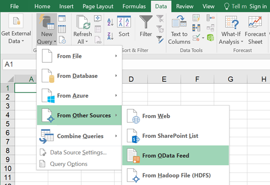
Go to Data > New Query > From Other Sources > From OData Feed.
Entering OData URL
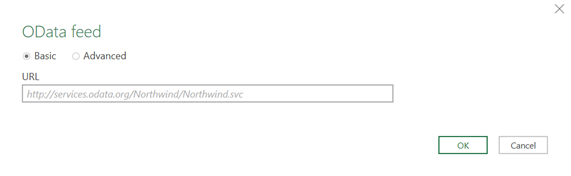
Select Basic and enter your OData URL.
Authentication (if relevant)
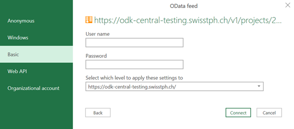
If you encounter a permissions prompt – commonly during the first-time setup of the connection or depending on the access level you previously selected – please follow these instructions to securely establish the connection:
- navigate to the Basic tab.
- input your ODK Central credentials (User name, Password).
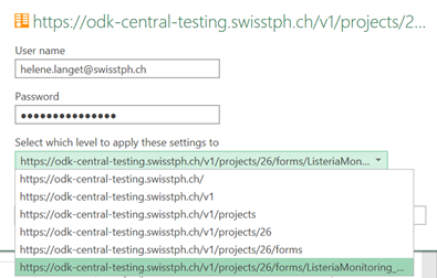
- select the level of the URL level you want to give permission for (Select which level to apply these settings to). This involves selecting the appropriate scope for the permissions—whether for the entire ODK Central server, just the specific project that includes your form, or exclusively for the form itself. This step ensures that permissions are accurately matched to your needs.
- click Connect to finalise the authentication process.
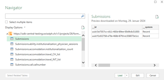
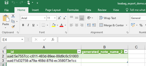
Selecting data to download
You have the flexibility to download either a single dataset or multiple datasets from an ODK form. Typically, an ODK form generates a primary submission dataset along with additional repeat datasets, where applicable.
- For a single item
- Select the dataset you wish to download
- Click Load (or Load To)
- A table will be created in a new worksheet (Load) or in the specified worksheet (Load To)
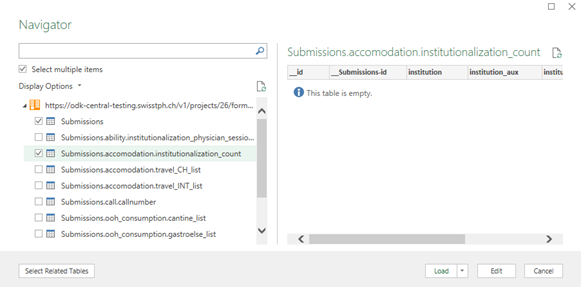
- For multiple items
- Enable the corresponding checkbox (Select multiple items)
- Select the datasets you are interested in
- Click Load (or Load To) for further actions. Selecting Load will only create connections, not tables.
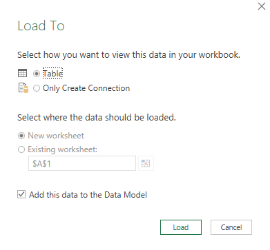
To manually allocate tables to a specific worksheet, follow these steps:
- Click on the arrow next to Load to unveil additional choices.
- Select Load To from the drop-down menu.
- Opt for Table to visualise the data as a table.
- Choose New worksheet or an Existing Worksheet.
Handling ODK variables within a group
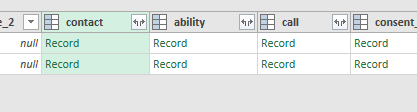
By default, ODK variables organised within a group (begin_group and end_group syntax) in the ODK form are not immediately visible upon loading.
To view and expand these grouped variables for analysis:
- Select the table you want to edit.
- Go to the Query tab that should have appeared as part of the tool ribbon.
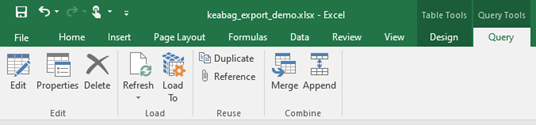
- Select Edit to open the Power Query Editor, where you can modify your dataset.
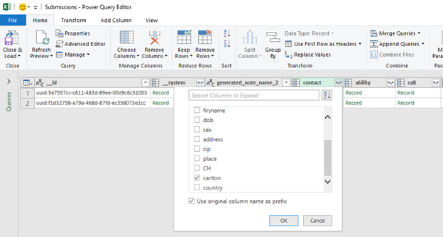
- In the Power Query Editor, look for the column that represents your grouped variables. Click on the double expansion arrows next to the group column name
 to reveal the grouped variables.
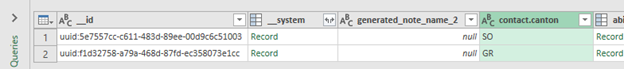
- A menu will appear, allowing you to choose which variables within the group you wish to display. After making your selections, click OK to confirm.
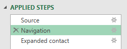
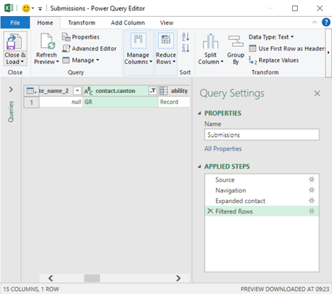
- The Power Query Editor tracks every modification in the Applied Steps section. Here, you can review all changes made to your dataset. If you need to adjust which variables are displayed from the group, you can return to the initial Navigation step and replace the expansion process to include additional (or remove) variables.
- Once you are satisfied with the selection of grouped variables, finalize your adjustments by clicking Close and Load. This action will apply your changes to the worksheet, integrating the expanded group data for further use.
Filtering data for customized views
Filtering data within the query allows for the creation of tailored views of your dataset, which can be organized across various worksheets for easy access and comparison. Follow these steps to implement data filtering within your queries:
- Open the Power Query Editor.
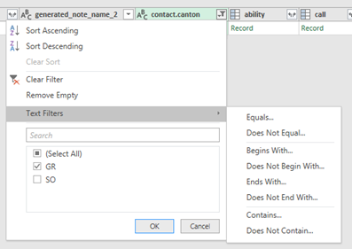
- Locate the column you wish to filter.
- Click the drop-down arrow in the column header to reveal the filtering options.
- You can choose to filter by specific values, range, or conditions based on your analysis needs (standard Excel filters).
To create a variety of tailored views from your dataset
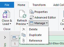
- Start with a base or reference query
- For each desired view, go to Manage, then Duplicate to replicate the reference query. This approach preserves the original query for further use.
- On each duplicated query, implement the specific filter settings you require. Make sure to review the sequence of applied steps to ensure accuracy and consistency in data representation.
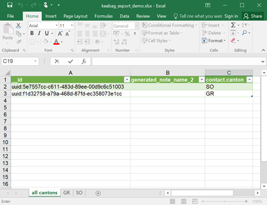
Note that each filtered view is linked to the original data source. Any updates or changes to the source data can be reflected in your filtered views by refreshing the queries. This process allows you to maintain various filtered views within separate queries, which can then be loaded into different worksheets for a comprehensive analysis, for instance hereafter creating a first worksheet with the full dataset, then subsequent datasets filtered by specific geographic area.
Manually refreshing data
Option 1 – using the Data tab
- Navigate to the Data tab on the ribbon.
- In the Data tab, click on the Refresh All icon.
Option 2- using the Design tab
- Select your table.
- Navigate to the Design tab on the ribbon.
- In the Data tab, click on the Refresh icon.
This action may prompt for your credentials if the connection has been stopped for some reason.
Automatically refreshing data
To ensure your dataset remains up-to-date without manual intervention, configure it for automatic refreshes.
Option 1 – using the Data tab
- Navigate to the Data tab on the ribbon.
- In the Data tab, click on the arrow next to Refresh All.
- Select Connection Properties in the drop-down menu
Option 2 – using the Design tab
- Select your table.
- Navigate to the Design tab on the ribbon.
- In the Design tab, click on the arrow next to Refresh.
- Select Connection Properties in the drop-down menu
Final steps for both options
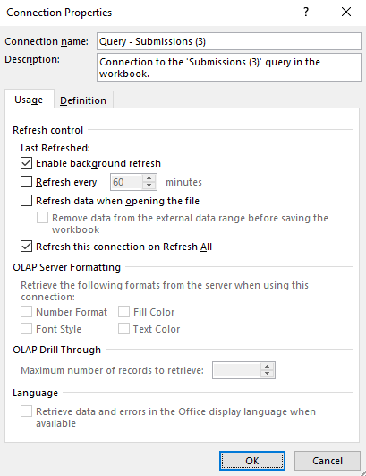
- In the Connection Properties dialog, navigate to the Refresh Control section. Here, you can enable and set the frequency of automatic refreshes according to your needs
- After configuring the settings for automatic refresh, click OK to save your changes and close the dialog.
Sharing the Excel file with third-parties without the OData connection
To distribute an Excel file containing data from an OData service URL while ensuring the connection to the live OData feed is removed, follow these structured steps. This approach ensures that the data remains available in the Excel file as static content (i.e., the link to the live OData feed is deleted, preventing updates or access to the original data source by the recipients).
Preparation
- Before removing the connection, make sure to refresh the data to its most current state, if necessary. Once the connection is removed, you will not be able to update the data automatically from the source.
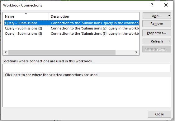
Option 1 – using the Data tab
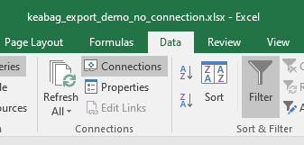
- Navigate to the Data tab on the ribbon.
- Click on Connections. This action will open a new window showing all the data connections in the Excel file.
- Click on the connection you wish to remove and select Remove. Confirm the removal if prompted. This action does not delete the data already downloaded and displayed in your Excel file; it merely removes the Excel's ability to refresh the data from the OData source.
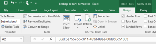
Option 2 – using the Design tab
- Select your table.
- Navigate to the Design tab on the ribbon.
- Click on Unlink.
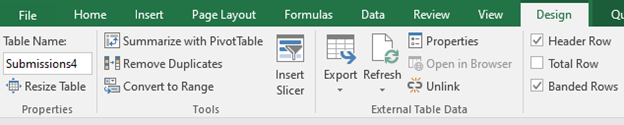
- Confirm the OData link deletion.
Finalisation
- After removing the connection, save your Excel file. This ensures that the data remains in Excel as static information, devoid of its live link to the OData source.
- Check that data are appropriately de-identified in accordance with relevant data protection regulations and ethical guidelines.
- Now, you can share the Excel file with external parties. The data from the OData source will be present, but the recipients will not be able to refresh or access the original data source directly through the Excel file.